Change Of Variables
How-To w/ Step-by-Step Examples!

Sometimes changing variables will make a huge difference in our ability to evaluate an integral.

Jenn, Founder Calcworkshop ® , 15+ Years Experience (Licensed & Certified Teacher)

We’ve seen the power of changing variables with u-substitution in single variable calculus, as well as switching to:

• Polar Coordinates
• Cylindrical Coordinates, or
• Spherical Coordinates

for multiple integrals.

But what did these transformations do for us?

By making a change of variables, we went from an integral that was “hard” to evaluate to something that was “easier.”

And let’s be honest…

…making integration easier is always the goal.

So, wouldn’t it be nice if there was a more general method for changing variables in multiple integrals?

And the answer is found in the Jacobian transformation.

Let’s learn why that is.

Change Of Variables

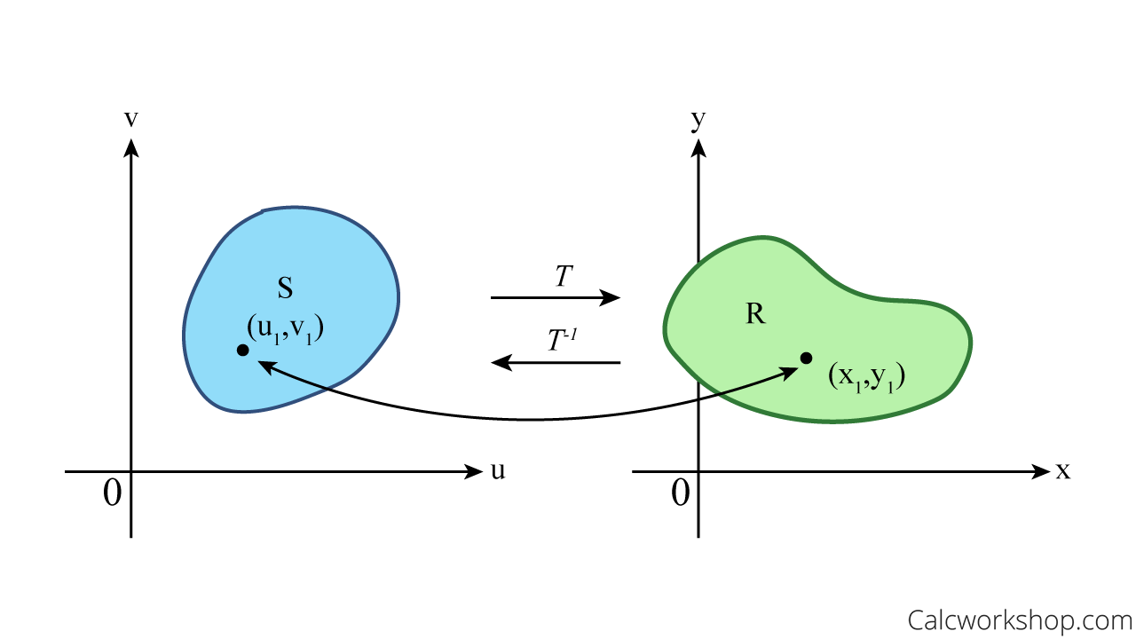
Okay, so in order to make a change of variables for multiple integrals, we must first consider the one-to-one transformation \(T\left( \right) = \left( \right)\) that maps a region \(S\) in the uv-plane onto a region \(R\) in the xy-plane.

This will then allow \(>\) to map region \(R\) in the xy-plane to region \(S\) in the uv-plane.

Using Change Of Variables And Transformation Maps

This means that the transformation \(T\) is just a function whose domain and range are both subsets of the real numbers in 2-space, which allows us to go back and forth from \(R\) to \(S\).

Why is that important?

Well, suppose region \(R\) in the xy-plane is “hard” to evaluate. In that case, we want to transform or change our region into something “easier” like the region \(S\) in the uv-plane, just like we did with u-substitution in single-variable calculus.

For instance, by changing variables, we can transform parallelograms into rectangles or ellipses into circles, which makes the region we are integrating over easier to handle.

Great. But how do we accomplish this?

By using the Jacobian method.

Jacobian Transformation

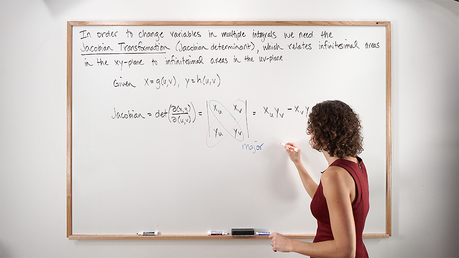
The Jacobian of the transformation \(T\) is given by:

\begin
\iint_ f(x, y) d A=\iint_ f(g(u, v), h(u, v))|J(u, v)| d u d v
\end

So, instead of integrating \(f\left( \right)\) over region \(R\), we will integrate over region \(S\) by making an appropriate change of variables and multiplying by the absolute value of the Jacobian Determinant.

Example – Jacobian Determinant

Let’s quickly look at an example of how we compute the Jacobian.

Find \(J\left( \right)\) when \(x = r\cos \theta \) and \(y = r\sin \theta \).

Well, the first thing we will do is find the first order partials with respect to \(r\) and \(\theta\) separately for both of our parametric equations.

\begin
\begin
x=r \cos \theta & y=r \sin \theta \\
\downarrow & \downarrow \\
\frac<\partial x><\partial r>=x_=\cos \theta & \frac<\partial y><\partial r>=y_=\sin \theta \\
\frac<\partial x><\partial \theta>=x_=-r \sin \theta & \frac<\partial y><\partial \theta>=y_=r \cos \theta
\end
\end

Now we place our partials into our determinant and evaluate.

\begin
J(r, \theta)=\left|\begin
\frac<\partial x> <\partial r>& \frac<\partial x> <\partial \theta>\\
\frac<\partial y> <\partial r>& \frac<\partial y><\partial \theta>
\end\right|
\end

\begin
=\left|\begin
\cos \theta & -r \sin \theta \\
\sin \theta & r \cos \theta
\end\right|
\end

\begin
=(\cos \theta)(r \cos \theta)-(-r \sin \theta)(\sin \theta)
\end

\begin
=r
\end

And now we have just proven why we must multiply by \(r\) when converting to polar coordinates and why the \(rdrd\theta \) makes sense!

Example – Change Of Variable In Multiple Integrals

Now that we know how to find the Jacobian, let’s use it to solve an iterated integral by looking at how we use this new integration method.

Ok, so the first thing we will do is sketch our region.

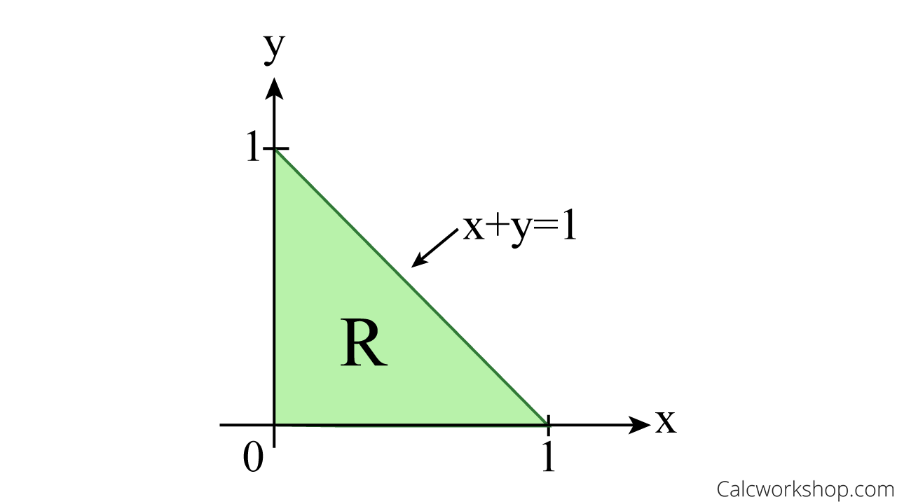
Sketch X Plus Y Equals 1 Cartesian Coordinates

Next, we will notice that our function \(f\left( \right) = >>> \right)>>\) is quite messy, and that without a suitable substitution trying to evaluate our double integral is going to be nigh impossible.

Time to make a change of variables.

So, looking more closely at our function \(>>> \right)>>\) we can let the numerator be:

\begin
u=x-y
\end

and

\begin
v=x+y
\end

But to change variables, we need to rewrite both \(x\) and \(y\) in terms of \(u\) and \(v\).

\begin
\begin
&u=x-y \\
&v=x+y
\end \Rightarrow \begin
&x=u+y \\
&y=v-x
\end \Rightarrow \begin
&x=u+(v-x) \\
&y=v-(u+y)
\end \Rightarrow \begin
&2 x=u+v \\
&2 y=v-u
\end \Rightarrow \begin
&x=\frac(u+v) \\
&y=\frac(v-u)
\end
\end

Now we have \(x = \frac\left( \right)\) and \(y = \frac\left( \right)\), which means we are now ready to find our Jacobian determinant.

\begin
J(u, v)=\left|\begin
\frac<\partial x> <\partial u>& \frac<\partial x> <\partial v>\\
\frac<\partial y> <\partial u>& \frac<\partial y><\partial v>
\end\right|
\end

\begin
=\left|\begin
\frac & \frac \\
-\frac & \frac
\end\right|
\end

\begin
=\left(\frac\right)\left(\frac\right)-\left(\frac\right)\left(-\frac\right)
\end

\begin
=\frac
\end

Next, we need to find our new limits of integration for \(u\) and \(v\).

We do this by substituting \(x = \frac\left( \right)\) and \(y = \frac\left( \right)\) into our region \(R\) domain and solving to obtain our new \(S\) region.

If \(x \ge 0\) and \(x = \frac\left( \right)\), then we can say \(\frac\left( \right) = 0\) or \(u = – v\).
If \(y \geq 0\) and \(y = \frac\left( \right)\), then we can say \(\frac\left( \right) = 0\) or \(u = v\).
If \(x + y \le 1\) and \(x = \frac\left( \right)\) and \(y=\frac(v-u)\), then we can say…

\begin
\frac(u+v)+\frac(v-u)=1 \text < or >v=1
\end

So, our new region looks like this:

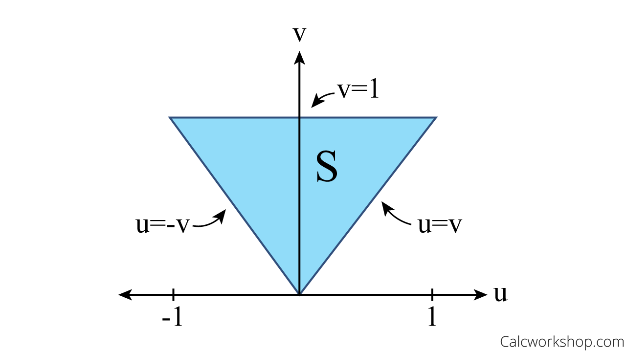
Uv Coordinates Region

And if we use horizontal slices, we obtain limit bounds as follows:

\begin
-v \leq u \leq v \text < and >0 \leq v \leq 1
\end

Finally, we’re ready to plug everything into our change of variables formula and evaluate.

\begin
\iint_ f(x, y) d A=\iint_ f(g(u, v), h(u, v))|J(u, v)| d u d v
\end

\begin
\iint_ e^<\left(\frac\right)> d A=\int_^ \int_^ e^<\left(\frac\right)>\left|\frac\right| d u d v
\end

\begin
\int_^\left(\int_^ \frac e^<\left(\frac\right)> d u\right) d v=\int_^\left(\left[\frac v e^<\left(\frac\right)>\right]_^\right) d v
\end

\begin
=\int_^\left(\frac v\left(e-e^\right)\right) d v=\left.\frac<\left(e-e^\right)> v^\right|_ ^
\end

\begin
=\frac
\end

See. We went from an impossibly “hard” integral to one that was “easier.”

3 Variable Jacobian

And a change of variables doesn’t just work for double integrals, but triple integrals too! The Jacobian transformation is defined similarly for a transformation of three variables where we will calculate the determinant using expansion by minors (cofactors).

If \(x = g\left( \right)\), \(y = h\left( \right)\), and \(z = k\left( \right)\) then

In fact, we use this particular Jacobian determinant for the three-variable transformation into spherical coordinates, thus yielding the Jacobian of \(\sin \phi \).

Now, changing variables can take a bit to get used to and isn’t for the faint of heart.

But don’t worry. We will work through examples in detail so you will get the hang of it in no time!

Video Tutorial w/ Full Lesson & Detailed Examples (Video)

Get access to all the courses and over 450 HD videos with your subscription

Monthly and Yearly Plans Available

Still wondering if CalcWorkshop is right for you?
Take a Tour and find out how a membership can take the struggle out of learning math.